How to make summarizing and reporting easy with Excel PivotTables
PivotTables are excellent tools to summarize and report large amounts of data. The only downside is that they require a lot of time to create, especially if the process needs to be repeated multiple times on different datasets. In this article, you’ll learn how to use Excel VBA and PivotTables to make summarizing and reporting easy and fast. You’ll also see how this can save you tons of time in the future when dealing with pivot tables, and will show you how to master both of these skills step-by-step with an example at the end of the article.
Set up a source data sheet
In order to create a PivotTable, you first need a source data sheet. This is simply a tab in your workbook that contains all of the raw data you want to summarize. To set up a source data sheet:
- Open a new workbook in Excel.
- Enter your data into the first sheet.
- Make sure each column has a heading, and that each piece of data is in its own cell.
Choose your fields
When you create a PivotTable, you’ll need to choose which fields you want to include. You can include as many or as few fields as you want, but generally speaking, the more fields you include, the more detailed your data will be.
To choose fields, simply click on the checkbox next to the field name. By default, all fields are selected, so if you only want to include certain fields, be sure to uncheck the ones you don’t want.
Add table calculations
You can use table calculations to show the total value of a field, the average value of a field, the number of unique values in a field, the minimum or maximum value in a field, and more. To add a table calculation:
- Select the field you want to calculate.
- Click the down arrow next to the field name, and then click Add Field Calculation.
- In the pop-up window that appears, enter your formula in the text box below Calculate, or select one from those provided by clicking Browse.
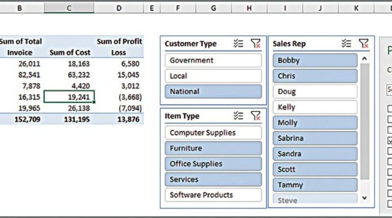
Create summary tables in the pivot table
With a pivot table, you can easily create summary tables that show counts, sums, or averages. You can also use them to filter and group data. To create a pivot table, first select the data you want to summarize. Then, click the Insert tab and choose PivotTable. In the Create PivotTable dialog box, choose where you want the pivot table to be placed. Lastly, choose which fields you want to include in the pivot table.
Organize fields, rows and columns
PivotTables are a powerful tool in Excel that can help you quickly summarize, analyze and report on data. To create a PivotTable, first select the data you want to include in the table. Then, go to the Insert tab and click on PivotTable. In the resulting dialog box, choose where you want to place the PivotTable and whether you want to use an existing worksheet or create a new one.
– Format it for maximum readability
Excel PivotTables are a powerful tool that can help you summarize and report data. They are easy to use and can save you time and effort when summarizing data. Here is a step-by-step guide on how to use PivotTables in Excel
1) Select the range of cells containing the data you want to summarize.
2) Click Insert > Tables > PivotTable
3) Drag fields into the Row Labels or Column Labels areas. You may also drag fields into the area labeled Values. You may need to drag fields from other worksheets or workbooks into this area if they are not already there.